If It Feels Hard to Read, It Probably Is

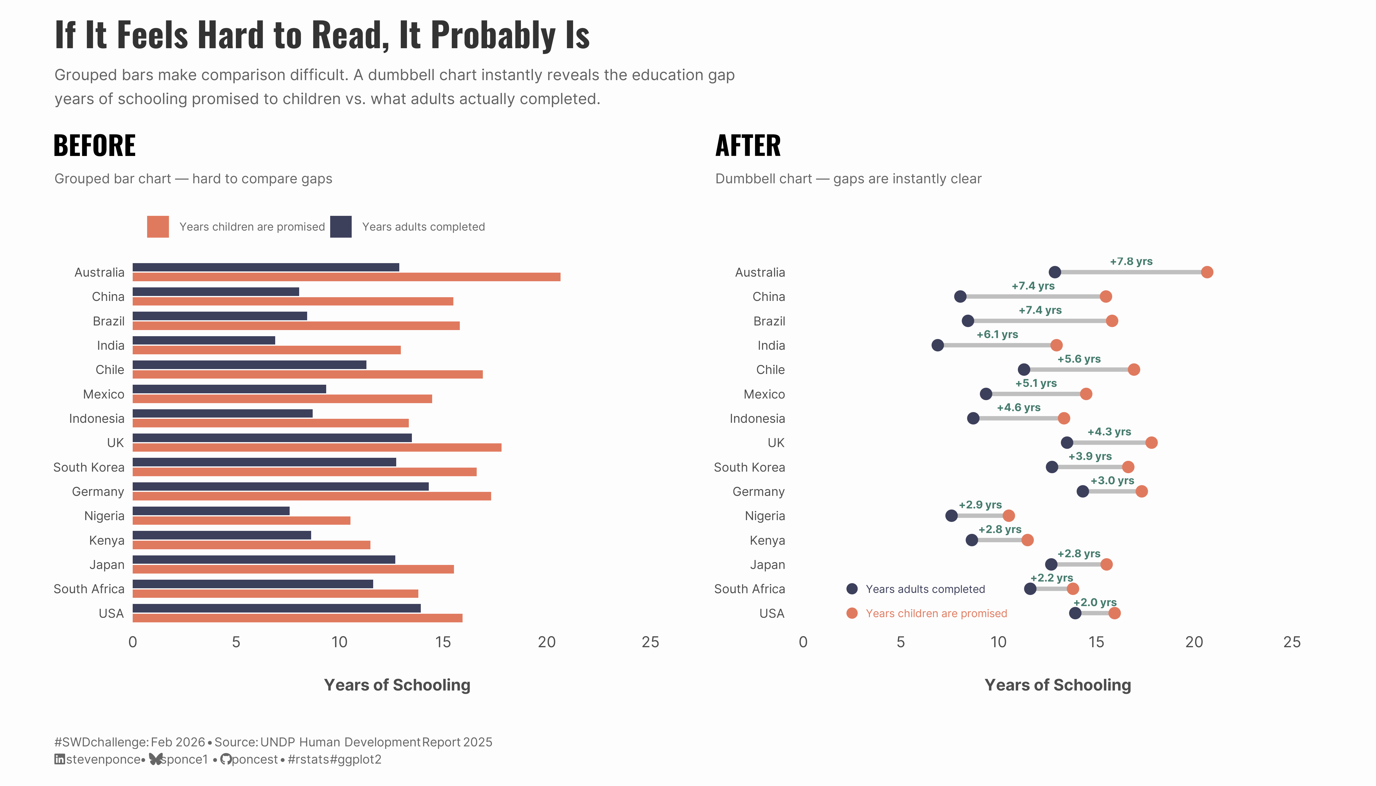
Grouped bars make comparison difficult. A dumbbell chart instantly reveals the education gap – years of schooling promised to children vs. what adults actually completed.

SWDchallenge

2026

A before-and-after visualization demonstrating the SWD lesson ‘Trust Your Instincts’ from Chapter 5 of storytelling with data: before & after. When comparing paired values across many categories, grouped bar charts create visual clutter. Switching to a dumbbell chart makes the education gap between expected and actual years of schooling instantly clear.

Author

Steven Ponce

Published

February 1, 2026

Challenge

This month’s challenge invites you to share your favorite SWD-inspired tip or lesson and bring it to life through a visual. Create something new or highlight an SWD example that illustrates it well.

Additional information can be found HERE

Visualization

Figure 1: Before-and-after comparison of the same education data. The left panel shows a grouped bar chart comparing expected vs. actual years of schooling across 15 countries — the paired bars make it hard to compare gaps. The right panel shows the same data as a dumbbell chart, where connected dots instantly reveal the education gap for each country. Australia, China, and Brazil have the largest gaps (7+ years), while USA, South Africa, and Japan have the smallest (around 2-3 years). The visualization demonstrates the SWD lesson: if a chart feels hard to read, try a different format.

Steps to Create this Graphic

1. Load Packages & Setup

Show code

```{r}
#| label: load

if (!require("pacman")) install.packages("pacman")
pacman::p_load(
tidyverse, ggtext, showtext, janitor,
  scales, glue, readxl, patchwork
)

### |- figure size ---- 
camcorder::gg_record(
  dir    = here::here("temp_plots"),
  device = "png",
  width  = 14,
  height = 8,
  units  = "in",
  dpi    = 320
)

# Source utility functions
suppressMessages(source(here::here("R/utils/fonts.R")))
source(here::here("R/utils/social_icons.R"))
source(here::here("R/utils/image_utils.R"))
source(here::here("R/themes/base_theme.R"))
```

2. Read in the Data

Show code

```{r}
#| label: read

hdi_url   <- "https://hdr.undp.org/sites/default/files/2025_HDR/HDR25_Statistical_Annex_HDI_Table.xlsx"
temp_file <- tempfile(fileext = ".xlsx")
download.file(hdi_url, temp_file, mode = "wb")

hdi_raw <- read_excel(temp_file, skip = 5) |>
  clean_names()

### |- Data Source ----
# Primary Source: UNDP Human Development Report 2025
# URL: https://hdr.undp.org/sites/default/files/2025_HDR/HDR25_Statistical_Annex_HDI_Table.xlsx
# Date Accessed: February 1, 2026
# Table: Statistical Annex Table 1 - Human Development Index and components
# Variables: Expected years of schooling, Mean years of schooling
# Documentation: https://hdr.undp.org/data-center/documentation-and-downloads
```

3. Examine the Data

Show code

```{r}
#| label: examine
#| include: true
#| eval: true
#| results: 'hide'
#| warning: false

glimpse(hdi_raw)
skimr::skim_without_charts(hdi_raw) 
```

4. Tidy Data

Show code

```{r}
#| label: tidy

education_data <- hdi_raw |>
  select(
    country,
    expected_years = years_7,
    actual_years   = years_9
  ) |>
  mutate(actual_years = as.numeric(actual_years)) |>
  filter(
    !is.na(country),
    !is.na(expected_years),
    !is.na(actual_years),
    !str_detect(country, "development$|OECD|countries$|World")
  )

selected_countries <- c(
  "Australia", "Germany", "United Kingdom", "United States", "Japan", "Korea (Republic of)",
  "Chile", "Mexico", "Brazil", "China",
  "Indonesia", "India", "South Africa",
  "Nigeria", "Kenya"
)

education_plot <- education_data |>
  filter(country %in% selected_countries) |>
  mutate(
    country = case_when(
      country == "Korea (Republic of)" ~ "South Korea",
      country == "United Kingdom" ~ "UK",
      country == "United States" ~ "USA",
      TRUE ~ country
    ),
    gap = expected_years - actual_years,
    gap_mid = (expected_years + actual_years) / 2,
    gap_lab = paste0("+", sprintf("%.1f", gap), " yrs")
  ) |>
  arrange(desc(gap)) |>
  mutate(country = factor(country, levels = rev(country)))

education_long <- education_plot |>
  select(country, expected_years, actual_years) |>
  pivot_longer(
    cols      = c(expected_years, actual_years),
    names_to  = "measure",
    values_to = "years"
  ) |>
  mutate(
    # Self-explanatory legend labels
    measure = recode(
      measure,
      expected_years = "Years children are promised",
      actual_years   = "Years adults completed"
    ),
    measure = factor(measure, levels = c("Years children are promised", "Years adults completed"))
  )
```

5. Visualization Parameters

Show code

```{r}
#| label: params

### |-  plot aesthetics ----
colors <- get_theme_colors(
  palette = list(
    expected   = "#E07A5F",
    actual     = "#3D405B",
    connector  = "gray75",
    gap_text   = "#457B6D"
  )
)

### |-  titles and caption ----
title_text <- "If It Feels Hard to Read, It Probably Is"

subtitle_text <- str_glue(
  "Grouped bars make comparison difficult. A dumbbell chart instantly reveals the education gap\nyears of schooling promised to children vs. what adults actually completed."
)

caption_text <- create_swd_caption(
  year = 2026,
  month = "Feb",
  source_text = "UNDP Human Development Report 2025"
)

### |-  fonts ----
setup_fonts()
fonts <- get_font_families()

### |-  plot theme ----
# Start with base theme
base_theme <- create_base_theme(colors)

# Add weekly-specific theme elements
weekly_theme <- extend_weekly_theme(
  base_theme,
  theme(
    # Text styling
    plot.title = element_text(
      face = "bold", family = fonts$title, size = rel(1.4),
      color = colors$palette$title, margin = margin(b = 10), hjust = 0
    ),
    plot.subtitle = element_text(
      family = fonts$subtitle, lineheight = 1.2,
      color = colors$palette$subtitle, size = rel(0.9), margin = margin(b = 20), hjust = 0
    ),
    
    ## Grid
    panel.grid = element_blank(),
    panel.grid.major.x = element_blank(),
    panel.grid.major.y = element_blank(),
    panel.grid.minor.x = element_blank(),
    panel.grid.minor.y = element_blank(),
    
    # Axes
    axis.title.x =  element_text(size = rel(0.9), color = "gray30", margin = margin(t = 20)),
    axis.title.y = element_text(size = rel(0.9), color = "gray30",  margin = margin(r = 20)),
    axis.text = element_text(color = "gray30"),
    # axis.text.y = element_text(size = rel(0.95)),
    axis.ticks = element_blank(),
    
    # Facets
    strip.background = element_rect(fill = "gray95", color = NA),
    strip.text = element_text(
      face = "bold",
      color = "gray20",
      size = rel(1),
      margin = margin(t = 8, b = 8)
    ),
    panel.spacing = unit(2, "lines"),
    
    # Legend elements
    legend.position = "right",
    legend.title = element_text(
      family = fonts$subtitle,
      color = colors$palette$text, size = rel(0.8), face = "bold"
    ),
    legend.text = element_text(
      family = fonts$tsubtitle,
      color = colors$palette$text, size = rel(0.7)
    ),
    legend.margin = margin(t = 0, r = 0, b = 0, l = 10),
    
    # Plot margin
    plot.margin = margin(10, 20, 10, 20)
  )
)

# Set theme
theme_set(weekly_theme)
```

6. Plot

Show code

```{r}
#| label: plot

### |- before plot ----
p_before <- ggplot(education_long, aes(x = country, y = years, fill = measure)) +
  # Geoms
  geom_col(position = position_dodge(width = 0.8), width = 0.7) +
  # Scales
  scale_fill_manual(
    values = c(
      "Years children are promised" = colors$palette$expected,
      "Years adults completed" = colors$palette$actual
    ),
    name = NULL
  ) +
  scale_y_continuous(
    limits = c(0, 25),
    breaks = seq(0, 25, 5),
    expand = expansion(mult = c(0, 0.02))
  ) +
  coord_flip(clip = "off") +
  # Labs
  labs(
    title = "BEFORE",
    subtitle = "Grouped bar chart — hard to compare gaps",
    x = NULL,
    y = "Years of Schooling"
  ) +
  # Theme
  theme(
    plot.subtitle = element_text(color = "gray40", size = 10),
    legend.position = "top",
    legend.justification = "left",
    legend.text = element_text(color = "gray40", size = 8),
    panel.grid.major.y = element_blank(),
    panel.grid.minor = element_blank(),
    axis.text.y = element_text(size = 9)
  )

### |- after plot ----
p_after <- ggplot(education_plot, aes(y = country)) +
  # Geoms
  geom_segment(
    aes(x = actual_years, xend = expected_years, yend = country),
    linewidth = 1.5,
    color = colors$palette$connector,
    lineend = "round"
  ) +
  geom_point(aes(x = actual_years), color = colors$palette$actual, size = 3.6) +
  geom_point(aes(x = expected_years), color = colors$palette$expected, size = 3.6) +
  geom_text(
    aes(x = gap_mid, label = gap_lab),
    color = colors$palette$gap_text,
    size = 2.8,
    family = fonts$text,
    fontface = "bold",
    vjust = -0.9
  ) +
  # Annotate
  annotate(
    "point",
    x = 2.5, y = 2,
    color = colors$palette$actual, size = 3.2
  ) +
  annotate(
    "text",
    x = 3.2, y = 2, label = "Years adults completed",
    color = colors$palette$actual, size = 2.8, hjust = 0, family = fonts$text
  ) +
  annotate(
    "point",
    x = 2.5, y = 1,
    color = colors$palette$expected, size = 3.2
  ) +
  annotate(
    "text",
    x = 3.2, y = 1, label = "Years children are promised",
    color = colors$palette$expected, size = 2.8, hjust = 0, family = fonts$text
  ) +
  # Scales
  scale_x_continuous(
    limits = c(0, 25),
    breaks = seq(0, 25, 5),
    expand = expansion(mult = c(0.02, 0.06))
  ) +
  # Labs
  labs(
    title = "AFTER",
    subtitle = "Dumbbell chart — gaps are instantly clear",
    x = "Years of Schooling",
    y = NULL
  ) +
  # Theme
  theme(
    plot.subtitle = element_text(color = "gray40", size = 10),
    panel.grid.major.y = element_blank(),
    panel.grid.minor = element_blank(),
    axis.text.y = element_text(size = 9)
  )

### |- combined plots ----
combined_plot <- (p_before | p_after) +
  plot_annotation(
    title = title_text,
    subtitle = subtitle_text,
    caption = caption_text,
    theme = theme(
      plot.title = element_text(
        size = rel(1.8),
        family = fonts$title,
        face = "bold",
        color = colors$title,
        lineheight = 1.15,
        margin = margin(t = 5, b = 5)
      ),
      plot.subtitle = element_text(
        size = rel(0.8),
        family = fonts$subtitle,
        color = alpha(colors$subtitle, 0.88),
        lineheight = 1.3,
        margin = margin(t = 5, b = 10)
      ),
      plot.caption = element_markdown(
        size = rel(0.65),
        family = fonts$subtitle,
        color = colors$caption,
        hjust = 0,
        lineheight = 1.4,
        margin = margin(t = 20, b = 5)
      ),
    )
  )
```

7. Save

Show code

```{r}
#| label: save

### |-  plot image ----  
save_plot_patchwork(
  combined_plot, 
  type = 'swd', 
  year = 2026, 
  month = 02, 
  width  = 14,
  height = 8,
  )
```

8. Session Info

Expand for Session Info

R version 4.4.1 (2024-06-14 ucrt)
Platform: x86_64-w64-mingw32/x64
Running under: Windows 11 x64 (build 26100)

Matrix products: default


locale:
[1] LC_COLLATE=English_United States.utf8 
[2] LC_CTYPE=English_United States.utf8   
[3] LC_MONETARY=English_United States.utf8
[4] LC_NUMERIC=C                          
[5] LC_TIME=English_United States.utf8    

time zone: America/New_York
tzcode source: internal

attached base packages:
[1] stats     graphics  grDevices datasets  utils     methods   base     

other attached packages:
 [1] here_1.0.1      patchwork_1.3.0 readxl_1.4.3    glue_1.8.0     
 [5] scales_1.3.0    janitor_2.2.0   showtext_0.9-7  showtextdb_3.0 
 [9] sysfonts_0.8.9  ggtext_0.1.2    lubridate_1.9.3 forcats_1.0.0  
[13] stringr_1.5.1   dplyr_1.1.4     purrr_1.0.2     readr_2.1.5    
[17] tidyr_1.3.1     tibble_3.2.1    ggplot2_3.5.1   tidyverse_2.0.0
[21] pacman_0.5.1   

loaded via a namespace (and not attached):
 [1] gtable_0.3.6       xfun_0.49          htmlwidgets_1.6.4  tzdb_0.5.0        
 [5] yulab.utils_0.1.8  vctrs_0.6.5        tools_4.4.0        generics_0.1.3    
 [9] curl_6.0.0         gifski_1.32.0-1    fansi_1.0.6        pkgconfig_2.0.3   
[13] ggplotify_0.1.2    skimr_2.1.5        lifecycle_1.0.4    compiler_4.4.0    
[17] farver_2.1.2       munsell_0.5.1      repr_1.1.7         codetools_0.2-20  
[21] snakecase_0.11.1   htmltools_0.5.8.1  yaml_2.3.10        pillar_1.9.0      
[25] camcorder_0.1.0    magick_2.8.5       commonmark_1.9.2   tidyselect_1.2.1  
[29] digest_0.6.37      stringi_1.8.4      rsvg_2.6.1         rprojroot_2.0.4   
[33] fastmap_1.2.0      grid_4.4.0         colorspace_2.1-1   cli_3.6.4         
[37] magrittr_2.0.3     base64enc_0.1-3    utf8_1.2.4         withr_3.0.2       
[41] timechange_0.3.0   rmarkdown_2.29     cellranger_1.1.0   hms_1.1.3         
[45] evaluate_1.0.1     knitr_1.49         markdown_1.13      gridGraphics_0.5-1
[49] rlang_1.1.6        gridtext_0.1.5     Rcpp_1.0.13-1      xml2_1.3.6        
[53] renv_1.0.3         svglite_2.1.3      rstudioapi_0.17.1  jsonlite_1.8.9    
[57] R6_2.5.1           fs_1.6.5           systemfonts_1.1.0

9. GitHub Repository

Expand for GitHub Repo

The complete code for this analysis is available in swd_2026_02.qmd. For the full repository, click here.

10. References

Expand for References

SWD Challenge:

Storytelling with Data: Feb 2026 - share your favorite SWD tip

Data Source: - United Nations Development Programme. (2025). Human Development Report 2025: Statistical Annex Table 1 - Human Development Index and components. Retrieved February 1, 2026, from https://hdr.undp.org/data-center/documentation-and-downloads

Book Reference: - Knaflic, C. N., Cisneros, A., & Velez, K. (2025). storytelling with data: before & after. Wiley. Chapter 5: Trust Your Instincts.

11. Custom Functions Documentation

📦 Custom Helper Functions

This analysis uses custom functions from my personal module library for efficiency and consistency across projects.

Functions Used:

fonts.R: setup_fonts(), get_font_families() - Font management with showtext
social_icons.R: create_social_caption() - Generates formatted social media captions
image_utils.R: save_plot() - Consistent plot saving with naming conventions
base_theme.R: create_base_theme(), extend_weekly_theme(), get_theme_colors() - Custom ggplot2 themes

Why custom functions?
These utilities standardize theming, fonts, and output across all my data visualizations. The core analysis (data tidying and visualization logic) uses only standard tidyverse packages.

Source Code:
View all custom functions → GitHub: R/utils